{
"cells": [
{
"cell_type": "raw",
"id": "9e1ef849",
"metadata": {},
"source": [
"---\n",
"format:\n",
" html:\n",
" include-in-header:\n",
" text: |\n",
" \n",
"---"
]
},
{
"cell_type": "markdown",
"id": "beff12c8",
"metadata": {},
"source": [
"# Ein Beispiel zur Stabilität von Gleitkommaarithmetik\n",
"\n",
"## Berechnung von $\\pi$ nach Archimedes\n"
]
},
{
"cell_type": "code",
"execution_count": null,
"id": "a7810264",
"metadata": {},
"outputs": [],
"source": [
"#| error: false\n",
"#| echo: false\n",
"#| output: false\n",
"using PlotlyJS, Random\n",
"using HypertextLiteral\n",
"using JSON, UUIDs\n",
"using Base64\n",
"\n",
"\n",
"## see https://github.com/JuliaPlots/PlotlyJS.jl/blob/master/src/PlotlyJS.jl\n",
"## https://discourse.julialang.org/t/encode-a-plot-to-base64/27765/3\n",
"function IJulia.display_dict(p::PlotlyJS.SyncPlot)\n",
" Dict(\n",
" # \"application/vnd.plotly.v1+json\" => JSON.lower(p),\n",
" # \"text/plain\" => sprint(show, \"text/plain\", p),\n",
" \"text/html\" => let\n",
" buf = IOBuffer()\n",
" show(buf, MIME(\"text/html\"), p)\n",
" #close(buf)\n",
" #String(resize!(buf.data, buf.size))\n",
" String(take!(buf))\n",
" end,\n",
" \"image/png\" => let\n",
" buf = IOBuffer()\n",
" buf64 = Base64EncodePipe(buf)\n",
" show(buf64, MIME(\"image/png\"), p)\n",
" close(buf64)\n",
" #String(resize!(buf.data, buf.size))\n",
" String(take!(buf))\n",
" end,\n",
"\n",
" )\n",
" end\n",
"\n",
" function Base.show(io::IO, mimetype::MIME\"text/html\", p::PlotlyJS.SyncPlot)\n",
" uuid = string(UUIDs.uuid4())\n",
" show(io,mimetype,@htl(\"\"\"\n",
" \n",
" \n",
"\"\"\"))\n",
"end "
]
},
{
"cell_type": "markdown",
"id": "8d4bd1ab",
"metadata": {},
"source": [
"Eine untere Schranke für $2\\pi$, den Umfang des Einheitskreises, erhält man durch die\n",
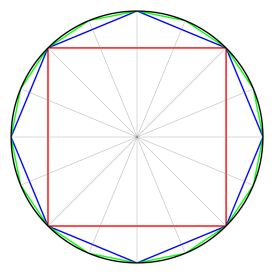
"Summe der Seitenlängen eines dem Einheitskreis eingeschriebenen regelmäßigen $n$-Ecks.\n",
" Die Abbildung links zeigt, wie man beginnend mit einem Viereck der Seitenlänge $s_4=\\sqrt{2}$ die Eckenzahl iterativ verdoppelt.\n",
"\n",
":::{.narrow}\n",
"\n",
"| Abb. 1 | Abb.2 |\n",
"| :-: | :-: |\n",
"|  |  |\n",
": {tbl-colwidths=\"[57,43]\"}\n",
"\n",
":::\n",
"\n",
"\n",
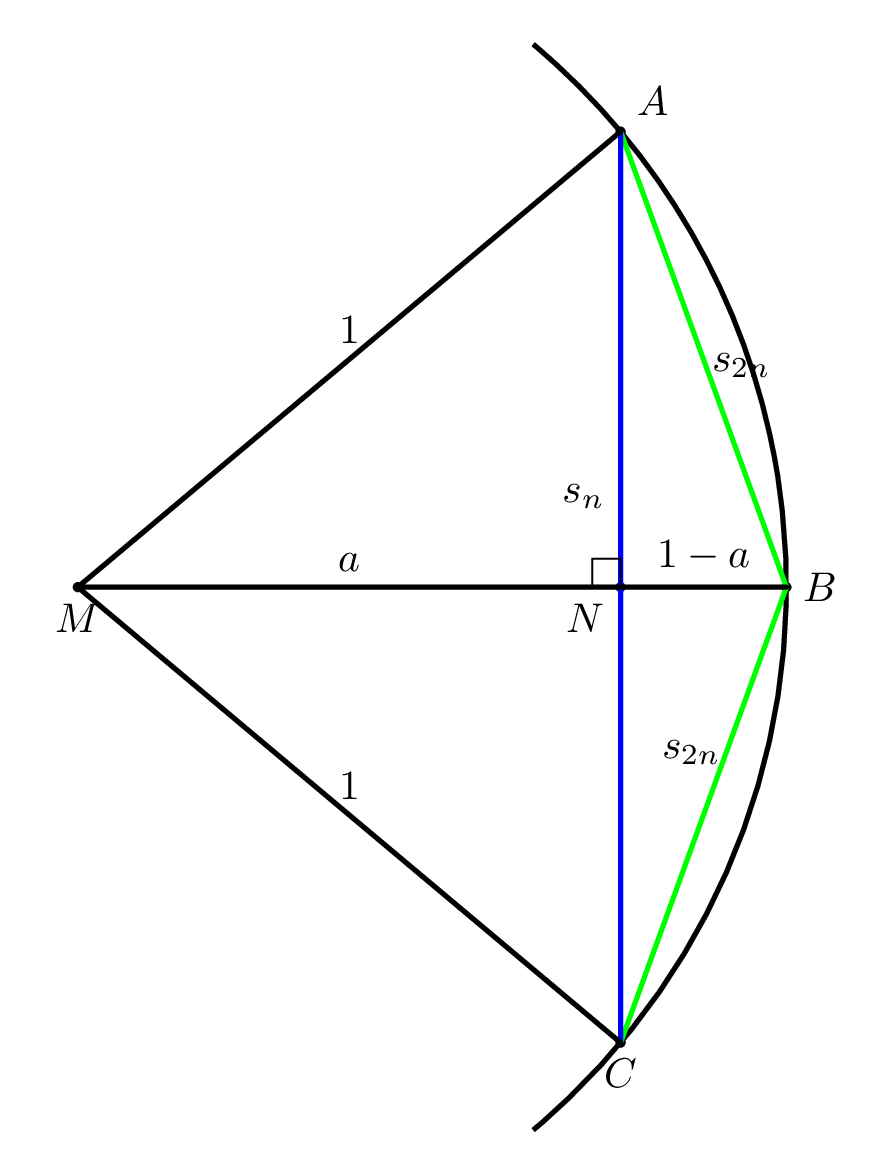
"Die zweite Abbildung zeigt die Geometrie der Eckenverdoppelung.\n",
"\n",
"Mit\n",
"$|\\overline{AC}|= s_{n},\\quad |\\overline{AB}|= |\\overline{BC}|= s_{2n},\\quad |\\overline{MN}| =a, \\quad |\\overline{NB}| =1-a,$ liefert Pythagoras für die Dreiecke $MNA$ und\n",
" $NBA$ jeweils\n",
"$$\n",
" a^2 + \\left(\\frac{s_{n}}{2}\\right)^2 = 1\\qquad\\text{bzw.} \\qquad\n",
" (1-a)^2 + \\left(\\frac{s_{n}}{2}\\right)^2 = s_{2n}^2\n",
"$$\n",
"Elimination von $a$ liefert die Rekursion\n",
"$$\n",
" s_{2n} = \\sqrt{2-\\sqrt{4-s_n^2}} \\qquad\\text{mit Startwert}\\qquad\n",
" s_4=\\sqrt{2}\n",
"$$\n",
"für die Länge $s_n$ **einer** Seite des eingeschriebenen regelmäßigen\n",
"$n$-Ecks.\n",
"\n",
"\n",
"Die Folge $(n\\cdot s_n)$\n",
"konvergiert monoton von unten gegen den\n",
"Grenzwert $2\\pi$:\n",
"$$\n",
" n\\, s_n \\rightarrow 2\\pi % \\qquad\\text{und} \\qquad {n c_n}\\downarrow 2\\pi\n",
"$$\n",
"Der relative Fehler der Approximation von 2π durch ein $n$-Eck ist:\n",
"$$\n",
" \\epsilon_n = \\left| \\frac{n\\, s_n-2 \\pi}{2\\pi} \\right|\n",
"$$\n",
"\n",
"\n",
"## Zwei Iterationsvorschriften^[nach: Christoph Überhuber, „Computer-Numerik“ Bd. 1, Springer 1995, Kap. 2.3]\n",
"Die Gleichung\n",
"$$\n",
" s_{2n} = \\sqrt{2-\\sqrt{4-s_n^2}}\\qquad \\qquad \\textrm{(Iteration A)}\n",
"$$\n",
"ist mathematisch äquivalent zu\n",
"$$\n",
" s_{2n} = \\frac{s_n}{\\sqrt{2+\\sqrt{4-s_n^2}}} \\qquad \\qquad \\textrm{(Iteration B)}\n",
"$$\n",
"\n",
"(Bitte nachrechnen!) \n",
"\n",
"\n",
"\n",
"Allerdings ist Iteration A schlecht konditioniert und numerisch instabil, wie der folgende Code zeigt. Ausgegeben wird die jeweils berechnete Näherung für π.\n"
]
},
{
"cell_type": "code",
"execution_count": null,
"id": "3f238690",
"metadata": {},
"outputs": [],
"source": [
"using Printf\n",
"\n",
"iterationA(s) = sqrt(2 - sqrt(4 - s^2))\n",
"iterationB(s) = s / sqrt(2 + sqrt(4 - s^2))\n",
"\n",
"s_B = s_A = sqrt(2) # Startwert \n",
"\n",
"ϵ(x) = abs(x - 2π)/2π # rel. Fehler \n",
"\n",
"ϵ_A = Float64[] # Vektoren für den Plot\n",
"ϵ_B = Float64[]\n",
"is = Float64[]\n",
"\n",
"@printf \"\"\" approx. Wert von π\n",
" n-Eck Iteration A Iteration B\n",
"\"\"\"\n",
"\n",
"for i in 3:35\n",
" push!(is, i)\n",
" s_A = iterationA(s_A) \n",
" s_B = iterationB(s_B) \n",
" doublePi_A = 2^i * s_A\n",
" doublePi_B = 2^i * s_B\n",
" push!(ϵ_A, ϵ(doublePi_A))\n",
" push!(ϵ_B, ϵ(doublePi_B))\n",
" @printf \"%14i %20.15f %20.15f\\n\" 2^i doublePi_A/2 doublePi_B/2 \n",
"end"
]
},
{
"cell_type": "markdown",
"id": "0c0178f5",
"metadata": {},
"source": [
"Während Iteration B sich stabilisiert bei einem innerhalb der Maschinengenauigkeit korrekten Wert für π, wird Iteration A schnell instabil. Ein Plot der relativen Fehler $\\epsilon_i$ bestätigt das:\n"
]
},
{
"cell_type": "code",
"execution_count": null,
"id": "f415aab0",
"metadata": {},
"outputs": [],
"source": [
"using PlotlyJS\n",
"\n",
"layout = Layout(xaxis_title=\"Iterationsschritte\", yaxis_title=\"rel. Fehler\",\n",
" yaxis_type=\"log\", yaxis_exponentformat=\"power\", \n",
" xaxis_tick0=2, xaxis_dtick=2)\n",
"\n",
"plot([scatter(x=is, y=ϵ_A, mode=\"markers+lines\", name=\"Iteration A\", yscale=:log10), \n",
" scatter(x=is, y=ϵ_B, mode=\"markers+lines\", name=\"Iteration B\", yscale=:log10)],\n",
" layout) \n"
]
},
{
"cell_type": "markdown",
"id": "02116ab2",
"metadata": {},
"source": [
"## Stabilität und Auslöschung\n",
"\n",
"Bei $i=26$ erreicht Iteration B einen relativen Fehler in der Größe des Maschinenepsilons:\n"
]
},
{
"cell_type": "code",
"execution_count": null,
"id": "3d50cba2",
"metadata": {},
"outputs": [],
"source": [
"ϵ_B[22:28]"
]
},
{
"cell_type": "markdown",
"id": "5ba088ba",
"metadata": {},
"source": [
"Weitere Iterationen verbessern das Ergebnis nicht mehr. Sie stabilisieren sich bei einem relativen Fehler von etwa 2.5 Maschinenepsilon:\n"
]
},
{
"cell_type": "code",
"execution_count": null,
"id": "2bcae61d",
"metadata": {},
"outputs": [],
"source": [
"ϵ_B[end]/eps(Float64)"
]
},
{
"cell_type": "markdown",
"id": "0bfd8235",
"metadata": {},
"source": [
"Die Form Iteration A ist instabil. Bereits bei $i=16$ beginnt der relative Fehler wieder zu wachsen.\n",
"\n",
"Ursache ist eine typische Auslöschung. Die Seitenlängen $s_n$ werden sehr schnell klein. Damit ist\n",
"$a_n=\\sqrt{4-s_n^2}$ nur noch wenig kleiner als 2 und bei der Berechnung von $s_{2n}=\\sqrt{2-a_n}$ tritt ein typischer Auslöschungseffekt auf.\n"
]
},
{
"cell_type": "code",
"execution_count": null,
"id": "365d4c27",
"metadata": {},
"outputs": [],
"source": [
"setprecision(80) # precision für BigFloat\n",
"\n",
"s = sqrt(BigFloat(2))\n",
"\n",
"@printf \" a = √(4-s^2) als BigFloat und als Float64\\n\\n\"\n",
"\n",
"for i = 3:44\n",
" s = iterationA(s)\n",
" x = sqrt(4-s^2)\n",
" if i > 20\n",
" @printf \"%i %30.26f %20.16f \\n\" i x Float64(x)\n",
" end \n",
"end\n"
]
},
{
"cell_type": "markdown",
"id": "04736a02",
"metadata": {},
"source": [
"Man sieht die Abnahme der Zahl der signifikanten Ziffern. Man sieht auch, dass eine Verwendung von `BigFloat` mit einer Mantissenlänge von hier 80 Bit das Einsetzen des Auslöschungseffekts nur etwas hinaussschieben kann. \n",
"\n",
"**Gegen instabile Algorithmen helfen in der Regel nur bessere, stabile Algorithmen und nicht genauere Maschinenzahlen!**\n",
"\n",
":::{.content-hidden unless-format=\"xxx\"}\n",
"\n",
"Offensichtlich tritt bei der Berechnung von $2-a_n$ bereits relativ früh\n",
"eine Abnahme der Anzahl der signifikanten Ziffern (Auslöschung) auf, \n",
"bevor schließlich bei der Berechnung von $a_n=\\sqrt{4-s_n^2}$ \n",
"selbst schon Auslöschung zu einem unbrauchbaren Ergebnis führt.\n",
"\n",
":::"
]
}
],
"metadata": {
"kernelspec": {
"display_name": "Julia 1.10.2",
"language": "julia",
"name": "julia-1.10"
}
},
"nbformat": 4,
"nbformat_minor": 5
}